
Modeling Plant Disease Epidemics: A Comprehensive Review of Disease Progress Curves
Temporal analysis of disease progression provides deeper insights into epidemiological patterns by examining disease levels across multiple time points. Disease progress curves (DPCs) capture how disease severity changes over time and reflect the combined effects of host, pathogen, and environment during an epidemic. Read more …

Temporal analysis of disease progression provides deeper insights into epidemiological patterns by examining disease levels across multiple time points. Disease progress curves (DPCs) capture how disease severity changes over time and reflect the combined effects of host, pathogen, and environment during an epidemic. Mathematical models such as Exponential, Logistic, Monomolecular, and Gompertz are commonly fitted to these curves to quantify epidemic development and compare outbreaks using indicators like fit statistics and parameter estimates. Disease severity may be measured once or repeatedly throughout the epidemic, and quantitative summaries such as Area Under Disease Progress Curves(AUDPC) and Area Under Disease Progress Stairs (AUDPS) help represent the overall disease burden. These metrics support effective comparison among epidemics. R programming, particularly through tools like the epifitter package, enables efficient modeling, visualization, and analysis of DPCs. Overall, disease progress curves are essential in agriculture, helping researchers and epidemiologists to monitor plant health, understand epidemic behavior, and improve disease management strategies.
Disease progress curves, Temporal disease analysis, Mathematical model fitting, R programming, AUDPC
![]()
![]()
![]()
1 Introduction
The challenge of maintaining food security has been increasingly affected by unpredictable climate changes and demanding crop environments. These persistent conditions lead to uncontrollable outbreaks of severe crop diseases over extended periods. Biotic constraints pose a significant threat to crop growth, impacting production and ultimately food security. These constraints often induce plant diseases that progress in a non-linear pattern, emphasizing the importance of timely intervention for effective management. A comprehensive investigation into underlying epidemics can significantly influence disease management practices. Employing suitable models to represent disease progression and predict its future development can greatly assist researchers in devising prompt management strategies. Analyzing the patterns, causes, and effects of diseases in plant populations is the central focus of epidemiological studies (Zadoks and Schein 1980; Van der Plank 1963). Examining disease progression curves helps researchers understand the timing of outbreaks and spread, ultimately leading to improved forecasting and management practices (Campbell and Madden 1990; Madden, Hughes, and Van den Bosch 2007). With recent improvements in statistical modeling and computational tools, analyzing disease progress curves has become more accurate and detailed. Applying non-linear regression models and temporal analysis has enhanced disease forecasting and risk assessment (Jeger 2004). Despite these advancements, there remains a need for comprehensive studies that integrate various epidemiological factors into a unified framework for specific plant diseases (Kranz 2003; Xu 2006). The disease progress curve is an essential tool for visually representing the proportion of diseased plants, providing a clear measure of a disease’s advancement. This curve effectively illustrates the influence of epidemiological factors and epidemic components, assisting researchers in identifying underlying epidemics (Campbell and Madden 1990; Madden, Hughes, and Van den Bosch 2007). Through the incorporation of appropriate mathematical models and thorough analysis of temporal progress, disease severity can be accurately quantified, enabling assessment of epidemic development and prediction of future disease trajectories (Van der Plank 1963; Hau and Kranz 1990). Employing statistical tools and visualization techniques is crucial for obtaining valuable insights into disease development and offers a convenient means of interpreting causal factors, thereby facilitating the timely implementation of effective management strategies to maintain healthy field conditions (Nutter Jr and Schultz 1995; Jeger and Viljanen-Rollinson 2001).
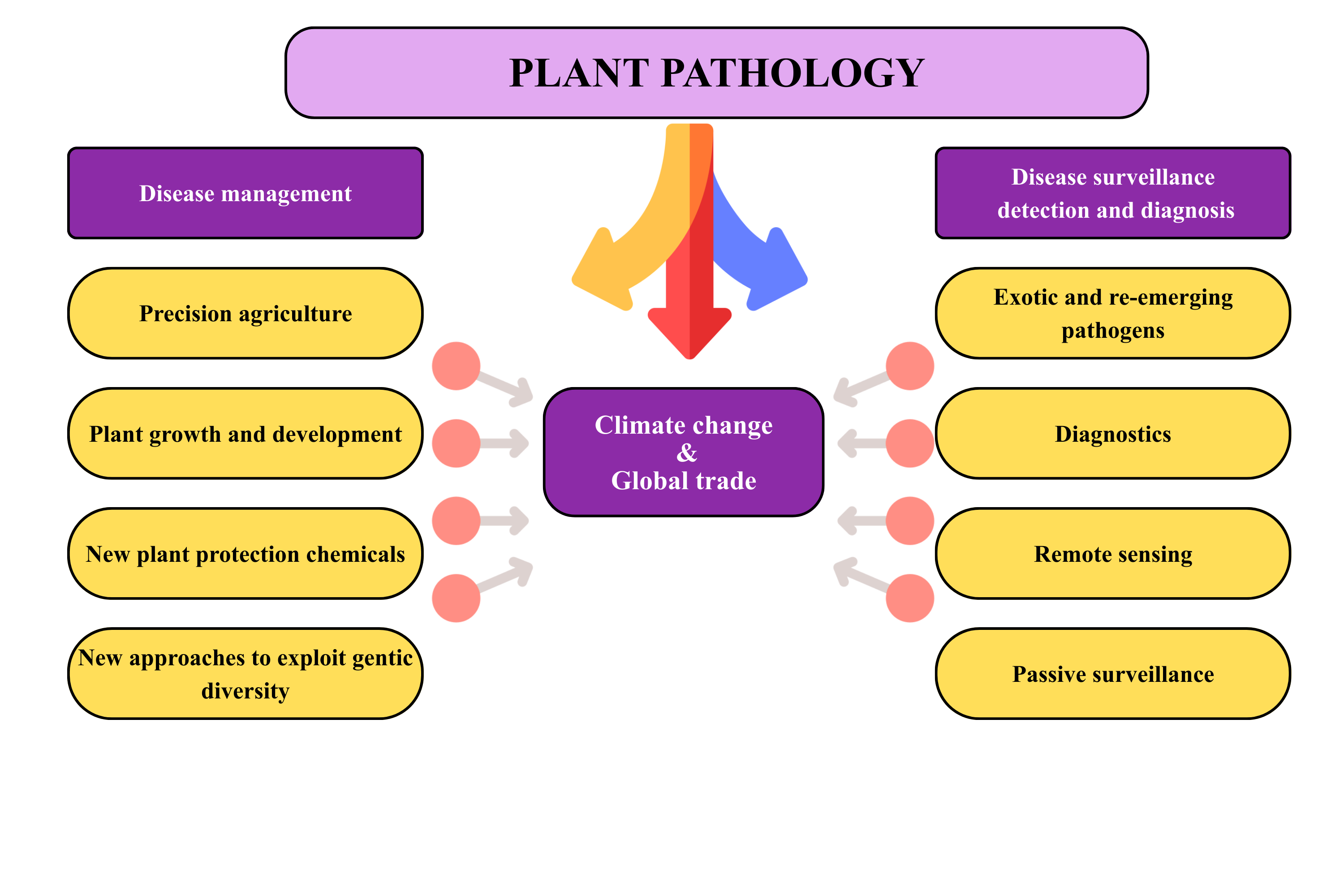
The interconnected nature of epidemiology, disease management, and global drivers such as climate change and trade is conceptually illustrated in Figure 1. This framework highlights how surveillance, diagnostics, and management strategies are shaped by evolving environmental and economic pressures, reinforcing the need for integrated approaches in plant pathology. A better understanding of the epidemic process is imperative for implementing an effective control strategy, as epidemiology and disease management are intertwined yet distinct and inseparable facets of plant pathology (Jeger 2004). Therefore, establishing an epidemiological framework using classical models and progress curves aims to target, enhance, and deploy methods that mitigate the risk of disease incidence in crops. Recently, (Savary and Willocquet 2020), has reinforced this need, showing that integrating epidemiological modelling with modern data driven approaches significantly improves disease forecasting and management outcomes in agricultural systems.
2 Nature of epidemics
Agriculture frequently results in simplified ecosystems in which humans alter the natural equilibrium between plants and pathogens. In this situation, diseases can develop into severe epidemics (González-Domı́nguez et al. 2020). The damage and loss incurred by crops are direct results of disease development, which occurs due to favorable conditions for initial infection and subsequent progression. These impacts and losses can be presented as the functions of disease progress. Plant disease epidemiology evolves by: a pathogen population, a plant host population, their environment, and human actions (Savary and Willocquet 2020). The quantification of derived functions is essential to comprehend disease progression and the factors impacting it. A thorough understanding of disease dynamics is important in epidemiological research, facilitating the timely implementation of management strategies through the visualization of disease progress curves.
2.1 Cyclic nature of plant disease
Plant disease epidemics exhibit a cyclic nature, characterized by recurring phases of pathogen development driven by interactions among the host, pathogen, and environment. The epidemic begins when inoculum-such as fungal spores, bacterial cells, nematodes, or virus particles transmitted by vectors-initiates infection and becomes established within susceptible host tissues. As the pathogen colonizes and multiplies within the host, it produces new inoculum capable of dispersing to additional infection sites, thereby sustaining the epidemic cycle. Diseases in which pathogens complete only one infection cycle during a crop cycle are classified as monocyclic, whereas pathogens capable of generating repeated infection cycles within the same season are described as polycyclic (Van der Plank 1963; Campbell and Madden 1990). Polycyclic pathogens often drive rapid epidemic development due to exponential inoculum build-up, while monocyclic pathogens progress more linearly, with epidemic intensity closely tied to the initial inoculum level (Madden, Hughes, and Van den Bosch 2007; Del Ponte 2023). Understanding these cyclic processes is fundamental for predicting epidemic dynamics and implementing timely disease management strategies.
3 Disease assessment
Disease assessment is the foundational step in plant disease epidemiology because every subsequent analysis- whether estimating infection rates, fitting disease progress models, or comparing treatments- depends on the accuracy and consistency of the initial measurements. The process begins with the identification of characteristic symptoms and signs, which requires familiarity with the pathogen, host physiology, and environmental conditions that influence symptom expression. (Campbell and Neher 1994) emphasized that although specific assessment techniques may vary depending on study objectives, the overarching goal remains constant: to obtain reliable, repeatable, and cost‑effective estimates of disease presence and intensity with known confidence.
A comprehensive disease assessment typically involves several sequential components. First, the sampling strategy must be defined, including the number of plants or plant parts to be evaluated, the spatial pattern of sampling within the field, and the timing of assessments relative to crop growth stages. Proper sampling ensures that the collected data accurately represent the true disease status of the population and minimizes bias caused by uneven disease distribution. the measurement of disease intensity is carried out using one or more standardized metrics. Disease intensity refers to the amount of disease within a defined area or population (Seem 1984). Within this framework, it is essential to distinguish between its major components:
• Disease incidence: which quantifies the proportion or number of plant units showing visible symptoms. It is particularly useful for diseases that produce discrete, easily identifiable symptoms.
• Disease severity: which measures the proportion of plant tissue affected, often expressed as a percentage of the total tissue area or volume (Kranz 1974). Severity is more informative for diseases that cause continuous damage, such as foliar blights or rusts.
In some cases, disease prevalence is also assessed, representing the proportion of fields or geographic units in which the disease occurs (Zadoks and Schein 1980). This metric is especially valuable for regional surveillance and risk mapping. Following measurement, the data must be recorded, validated, and standardized. This may involve the use of categorical scales, diagrammatic keys, digital imaging tools, or quantitative laboratory methods, depending on the disease and study objectives. Standardization reduces assessor bias and enhances comparability across observers, locations, and time points. Finally, the assessed data are summarized and interpreted to characterize the epidemic. These summaries form the basis for constructing disease progress curves, estimating epidemiological parameters, comparing treatments, and informing management decisions. Accurate disease assessment therefore not only describes the current status of disease but also enables robust modelling, forecasting, and evaluation of control strategies.
3.1 Methods of disease assessment
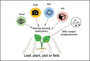
Disease assessment in crops is a fundamental component of plant pathology, serving as the basis for quantifying epidemic intensity, comparing treatments, evaluating host resistance, and developing reliable disease progress curves. Crop disease severity can be quantified through several methodological approaches that differ in precision, scalability, and practicality. Traditional visual assessment conducted by trained observers remains the most widely adopted technique due to its simplicity and suitability for field conditions; however, it is inherently subjective and susceptible to assessor bias, even when standardized scales are used (Nutter Jr and Schultz 1995; Bock et al. 2010). Advancements in imaging technologies have enabled the development of remote sensing-based assessment methods, including RGB imaging, multispectral imaging (MSI), and hyperspectral imaging (HSI), which significantly enhance objectivity and consistency. RGB cameras capture high-resolution colour imagery suitable for detecting visual symptoms, while MSI records reflectance in selected spectral bands associated with plant physiological responses and stress. HSI, providing detailed spectral signatures across numerous contiguous wavelengths, supports early detection of subtle biochemical and structural changes preceding visible symptom expression (Mahlein 2016; Mahlein et al. 2018). In addition to imaging-based approaches, contact-based measurement methods-such as manual lesion counting, digital area measurement tools, planimetry, and laboratory-based quantification of pathogen biomass using qPCR or ELISA-offer high accuracy but are often labour-intensive and time-consuming (Bock et al. 2010; Mutka and Bart 2015). Collectively, these methods form a continuum from simple field-based visual scoring to advanced sensor-driven analytics, allowing researchers to select the most appropriate approach based on the scale, objectives, and precision requirements of disease monitoring in agricultural systems (Del Ponte 2023). These diverse approaches to disease quantification—from visual scoring to advanced spectral imaging and contact-based measurements—are conceptually illustrated in Figure 2, which categorizes remote sensing and direct measurement techniques based on their mode of interaction with plant material.
A good-quality disease assessment should be reliable, meaning that it consistently reflects the true level of disease within a crop population. Reliability encompasses three key attributes: accuracy, precision, and reproducibility (Nutter Jr and Schultz 1995; Bock et al. 2010). Accuracy refers to the closeness of the sample mean to the true population mean, indicating how well an assessment represents actual disease levels. Precision, in contrast, measures how closely repeated estimates cluster around their mean value, commonly quantified using the sample variance (S²). A larger S² indicates lower precision, reflecting greater variability among assessment values; such variability may arise from assessor error or genuine heterogeneity in disease distribution among plants (Bock et al. 2010). Understanding the sources of variation is essential, as biological factors-such as localized pathogen spread or microenvironmental differences-can also contribute significantly to observed variance. Reproducibility is another critical component of reliable disease quantification and refers to an evaluator’s ability to consistently assign similar disease severity estimates when repeating assessments on the same plants or plots within a short period. One widely used approach to evaluate reproducibility involves correlation analysis between two consecutive assessments of identical units. A high correlation coefficient (r ≥ 0.80) is generally considered indicative of strong reproducibility, suggesting that the assessment protocol produces consistent and dependable results (Nita, Ellis, and Madden 2003; Nutter Jr and Schultz 1995). Ensuring high reproducibility is fundamental, as it increases confidence in treatment comparisons, model fitting, and epidemiological interpretations. In practical disease assessment, accuracy, precision, and reproducibility are achieved through the use of standardized rating scales, assessor calibration exercises, and repeated or replicated measurements, all of which reduce observer related variation and ensure that disease estimates reliably reflect true epidemic conditions.
4 Modeling the epidemics
The main goal of epidemiological research is to comprehend the correlation between disease patterns and external influences. The progression of a disease over time can be represented through appropriate models, often depicted as curves. Enhanced understanding can facilitate the creation of more effective, sustainable, and efficient management strategies to mitigate the impact of diseases on crop yield. The relationship between epidemic development and crop yield loss can be more accurately quantified by integrating disease progress with the timing of infection events. Traditional methods often rely solely on final disease severity or cumulative disease intensity; however, the timing of pathogen establishment has a critical influence on the final yield outcome. The framework proposed by the 1998 study on coupling disease-progress curves with time-of-infection functions demonstrated that early infections disproportionately reduce yield because they allow more time for pathogen colonization and physiological disruption of host tissues (Madden, Hughes, and Irwin 2000).
4.1 Disease progress curves
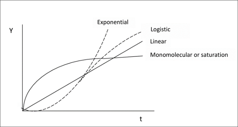
Disease intensity - expressed as incidence, prevalence, or severity- when monitored over time, produces disease progress curves (DPCs), which serve as fundamental tools for quantifying the temporal dynamics of plant disease epidemics. These curves capture how diseases evolve within a host population and allow researchers to analyze epidemic patterns using established growth models that reflect biological processes of infection, colonization, and host response (Jeger 2004; Madden, Hughes, and Van den Bosch 2007). Depending on the pathogen’s life strategy and environmental interactions, DPCs typically follow mathematical forms such as monomolecular, logistic, Gompertz, or exponential curves as illustrated in Figure 3, each corresponding to unique epidemic behaviors and contributing factors (Dar, Parry, and Bhat 2021; Esker, Savary, and McRoberts 2013). Quantitative analysis of these curves provides two critical epidemiological parameters: the initial inoculum level (y₀) and the apparent infection rate (r), both of which help characterize epidemic onset and progression (Nutter Jr, Eggenberger, and Littlejohn 2015; Jeger and Viljanen-Rollinson 2001). These parameters enable comparisons across cultivars, treatments, environments, and cropping systems, making them essential in evaluating the effectiveness of cultural practices, host resistance, and chemical or biological control measures (Del Ponte and Esker 2008; Esker, Savary, and McRoberts 2013). In addition to describing disease development, DPCs also hold substantial predictive value. Because disease severity patterns often correlate with future epidemic intensity, fitted progress curves can be used to forecast disease trajectories, epidemic thresholds, and potential yield impacts under varying environmental scenarios (Duku, Sparks, and Zwart 2016; Bock et al. 2020). This predictive capacity supports the development of early-warning systems and disease risk models that guide timely and effective management interventions, particularly in the context of climate variability and precision agriculture (Garrett et al. 2013; Mahlein 2016). Thus, disease progress curves serve not only as descriptive epidemiological tools but also as a foundation for forecasting, decision support, and sustainable plant disease management.
Disease dynamics are measured using disease intensities y(t), which can be depicted as summation curves or rate curves. A Disease Progression Curve (DPC) provides a summary of the interaction among the three primary components of the disease triangle during an epidemic. The shapes of the curves can exhibit significant variations based on the individual characteristics of each component. These characteristics can be influenced by management practices aimed at altering the trajectory of the epidemic, with the ultimate objective of restraining the progression of the disease.
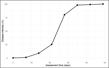
The disease progress curve illustrated in Figure 4 was generated using a model dataset representing disease severity recorded across successive time points (days). The visualization was produced using the R statistical computing environment (RStudio), which enabled the construction of a representative epidemic trajectory for demonstrating typical patterns of temporal disease development.
4.2 Classifiaction of epidemics
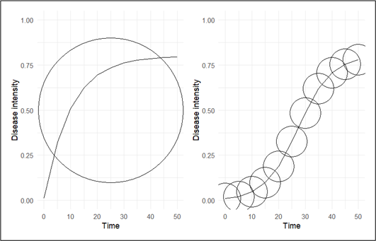
The morphology of disease progress curves (DPCs) exhibits significant variability depending on the type of crop disease. This diversity can be categorized into two primary groups: monocyclic and polycyclic (Del Ponte 2023). Monocyclic diseases involve disease progression and sustenance solely through the primary inoculum, with no secondary infection occurring during the crop cycle. Classic examples include common smut of maize (Ustilago maydis) and Fusarium wilt of banana (Fusarium oxysporum f. sp. cubense), both of which typically produce saturation‑type progress curves. In contrast, polycyclic diseases generate secondary inoculum within the same season, enabling repeated infection cycles. Well‑known examples include late blight of potato (Phytophthora infestans) and powdery mildew of cereals (Blumeria graminis), which characteristically produce sigmoid‑shaped progress curves due to rapid, exponential epidemic development. These distinct curve morphologies are visually represented in Figure 5.
The principal aim of epidemiological research is to decrease the incidence of disease below a specific threshold. Therefore, in order to comprehensively reduce the progression of diseases, it is imperative to develop distinct mathematical models for each type of disease. Monocyclic disease is primarily concerned on the amount of inoculum present at the begin of the infection stage(initial inoculum). The initial inoculum amount (Q1) at the beginning of the current season is the sum of the initial inoculum at the beginning of the previous season (Q0) and the increment resulting from the pathogen’s growth and development during the season as represented in Equation 1.
\[Q_{1} = Q_{0} + increment \tag{1}\]
The increment is directly proportional to the amount of last season’s initial inoculum. It can be approximated as a simple proportion of last season’s initial inoculum, KQ0, where K is a proportionality constant (Equation 2).
\[Q_{1} = Q_{0} + KQ_{0} \tag{2}\]
The K represents all the factors affecting the growth of the pathogen dispersal of inoculum and other factors contributing to the increase in inoculum. The value of K depends on various factors such as environmental conditions, cultivation practices, crop development. The value of K depends on the nature of disease progress , it will be positive and there is a net increase from one session to next . On the other hand if there is a net decrease in the production of inoculum, K would be negative, this situation occurs during rotation with non host crops. In order to describe the changes in the initial inoculum from one season to the next in a polyetic epidemic, we will generalize the subscript that indicates the season (Equation 3).
\[Q_{T+1} = Q_{T} + KQ_{T} \tag{3}\]
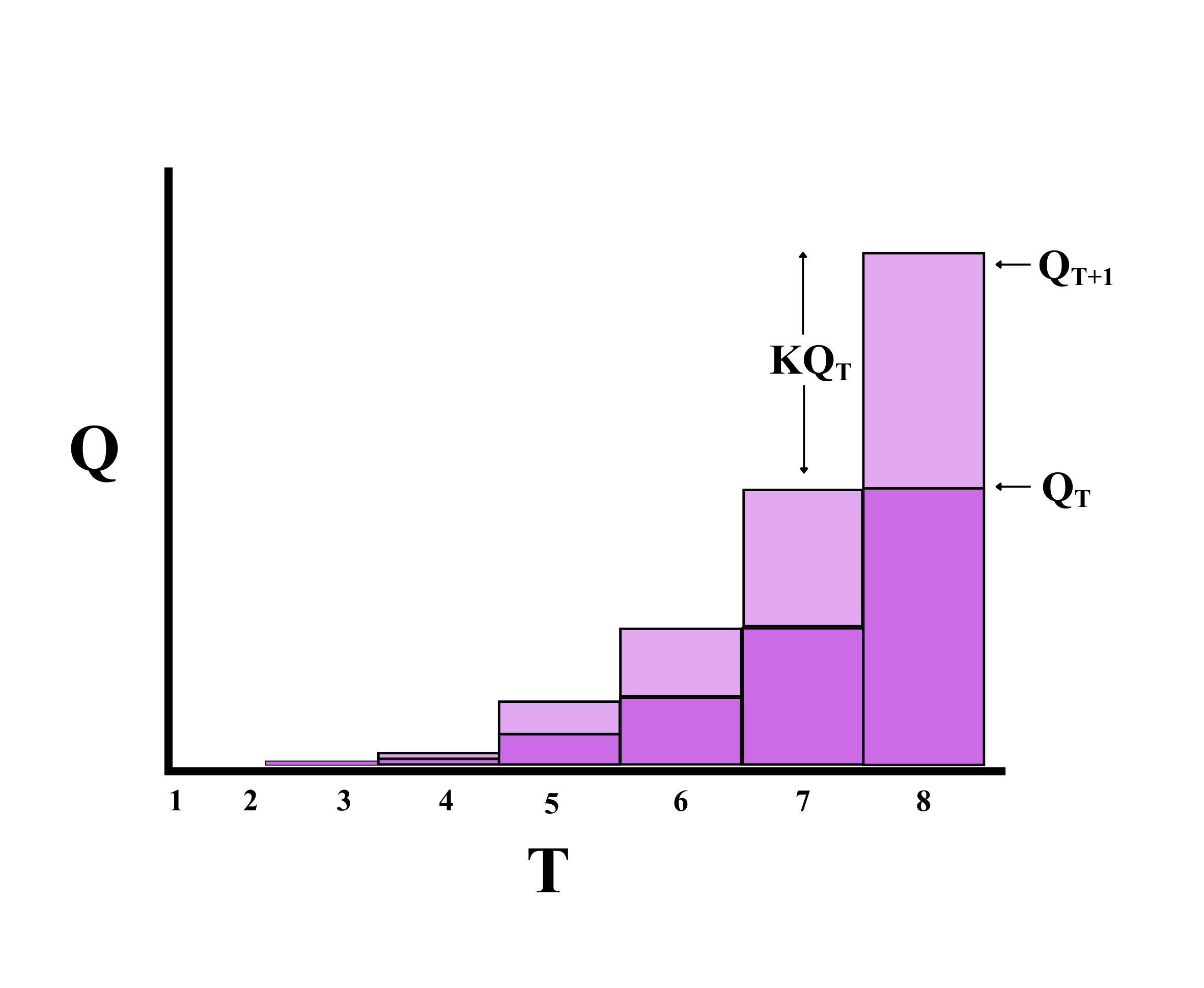
The progression of initial inoculum, governed by the proportionality constant K, is conceptually illustrated in Figure 6. The diagram demonstrates how inoculum quantity evolves between two consecutive time interval, emphasizing the role of K in determining net increase or decrease.
We solve the equation repeatedly, sequentially adjusting the subscript T, denoting time, as each consecutive season succeeds, and setting the current value of QT+1 as the value of QT in the subsequent season. To simplify the equation we include a constant K(representing an average value over many seasons). From the equation, if K is positive the graph curves upwards(as the light grey portion in the figure increases with increase in initial inoculum in the successive seasons).
In polycyclic diseases, consistent quantitative modeling is employed to analyze repetitive cycles occurring within multiple seasons. This method allows for the observation of these recurring cycles within the same season, ensuring thorough and comprehensive analysis. So the value of time here becomes days or weeks instead of years, and since the time unit is in weeks or days the increase in time is denoted by ΔT.
\[q_{T+ΔT}=q_{T}+q_{T}×k×ΔT \tag{4}\]
Here q represents the quantity of inoculum during the epidemic, and k represents the proportion by which inoculum increases over time. The units of k and T are measured in the same units. For instance, if time is measured in days, the units of k would be proportion per day. The production of inoculum typically happens sporadically during separate and distinct infection periods that vary in duration due to the weather. The value of k would probably vary for each infection period. To develop the most basic model feasible for effective application as a managerial instrument, we will modify the above model by standardizing the time frame and assuming a constant value for k. As shown in Equation 5 instead of accommodating varying k values based on environmental circumstances, we will use the average value of k across the entire epidemic period.
\[q_{T+ΔT}-q_{T}=q_{T}×k ×ΔT\]
The change in the amount of inoculum in one time step, Δq, is simply the difference between the amount of inoculum at time T and the amount of inoculum at time T+ΔT:
\[Δq=q_{T}×k×ΔT ;\]
\[∆q/ΔT=q_{T}×k \tag{5}\]
Now instead of advancing time in discrete steps, we will advance time continuously, making ΔT infinitesimally small:
\[dq/dt =q×k \tag{6}\]
Therefore, the rate of change in the quantity of inoculum is proportional to the quantity of inoculum at any point in time.
\[q = q_{0}e^{kt} \tag{7}\]
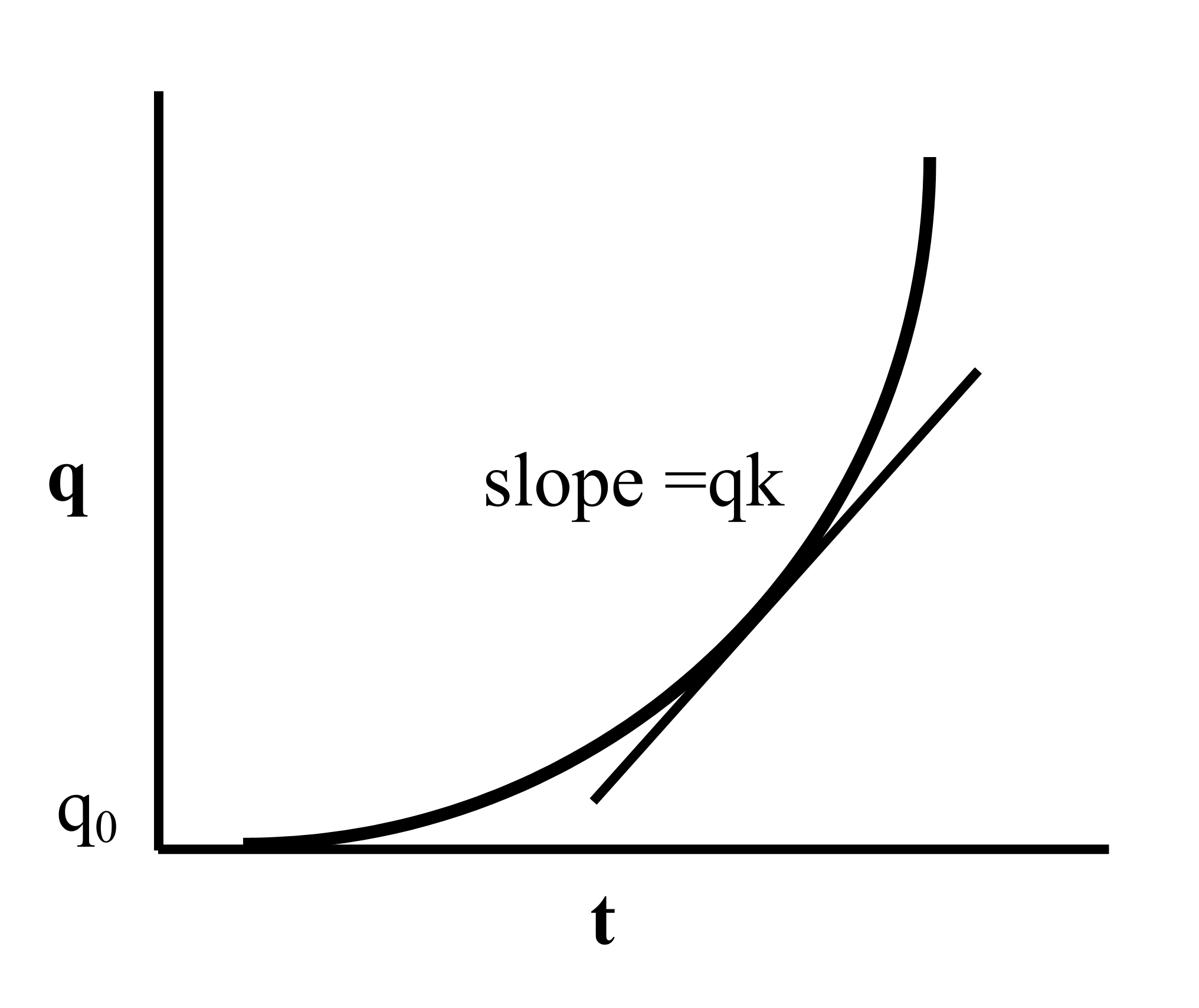
The given expression is analogous to an exponential function, with q0 representing the initial inoculum, and e as the base of the natural logarithm. The instantaneous rate of change in q is denoted by dq/dt, which signifies the slope of the tangent to the curve at any given point (Figure 7).
5 Population models of disease
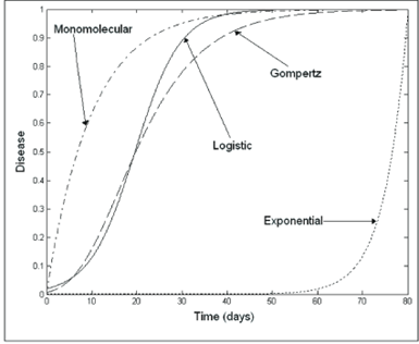
Mathematical models can be utilized to analyze DPC (Disease Progression Curve) data, enabling the expression of epidemic advancement in terms of rates and absolute or relative quantities. This approach involves employing population dynamics, or growth-curve, models, for which the estimated parameters typically hold biological significance and effectively depict epidemics that do not exhibit a decline in disease intensity (Savary and Willocquet 2020). The diversity in mathematical modeling approaches for disease progression is illustrated in Figure 8, which compares four commonly used growth-curve models and their respective trajectories over time. By fitting a suitable model to the progression curve data, researchers gain access to a distinct set of parameters, facilitating the representation, comprehension, and comparison of epidemics. The definition of an epidemic can be expressed in terms of dy/dt, where y represents disease severity or incidence and t represents time. The term dy/dt signifies the absolute rate of disease increase or absolute growth rate. Quantifying epidemics involves expressing dy/dt as a function of y, t, or other relevant variables (Madden, Hughes, and Van den Bosch 2007).
5.1 Exponential
The exponential model assumes that the absolute rate of disease increase (dy/dt) is proportional to the disease intensity (y). The differential equation for the exponential model is
\[dy/dt= r×y\] r is a rate parameter (units = time-1) and y is the disease intensity.
Biologically, this formulation suggests that diseased plants, or y, and r at each time contribute to disease increase. The value of dy/dt is minimal when y=0 and increases exponentially with the increase in y.
The integral for the exponential model is given by
\[y = y_{0}e^{rt} \tag{8}\]
yo is a constant of integration that also represents initial disease level, if one assumes that the epidemic starts at t = 0. Linearised exponential model = ln(y) = ln(yo) + rt. If r is constant, a plot of In(y) = (y) vs t is a straight line with slope r. The exponential model may be appropriate when there is no limitation to disease increase and this model is appropriate in the very early stages of epidemics (Bowen 2015).
5.2 Monomolecular
The monomolecular model operates under the assumption of a carrying capacity of one, meaning that the maximum disease level is one, and the severity or incidence of the disease is measured as a proportion. Diseased plant tissue is constrained to a range between zero (healthy) and one (complete disease). Additionally, the model assumes that the absolute rate of change is directly proportional to the healthy tissue, denoted as (1-y). The rate equation can be written as dy/dt = r(K - y) in which K is a parameter representing maximum disease level Ymax. Often the assumption is made that the maximum disease level equals = 1 (100%). The term (1 - y) represents disease-free plant tissue or the proportion of disease-free plants. This model commonly describes the temporal patterns of the monocyclic epidemics. In those, the inoculum produced during the course of the epidemics do not contribute new infections. Therefore, different from the exponential model, disease intensity does not affect the epidemics and so the absolute rate is proportional to 1 - y (Kebede and Golla 2020).
5.3 Logistic model
The logistic model represents a more comprehensive iteration of the preceding models, encompassing their combined features. Van der Plank (Van der Plank 1963) proposed a distinct type of logistic model, better suited for most polycyclic diseases, indicating the occurrence of secondary spread within a single growing season. This growth model stands as the most widely employed method for characterizing plant disease epidemics (Berger 1981). The differential equation of the logistic model can be written as;
\[\frac{dy}{dt} = ry(1 - y) \tag{9}\]
here “r” is the infection rate of the logistic model, y is the proportion of diseased individuals or host tissue and (1−y) is the proportion of non-affected individuals or host area. Biologically, y in its differential equation implies that dy/dt increases with the increase in y (as in the exponential) because more disease means more inoculum. However, (1−y) leads to a decrease in dy/dt. when y approaches the maximum y = 1, because the proportion of healthy individuals or host area decreases (as in the monomolecular). Therefore, dy/dt is minimal at the onset of the epidemics, reaches a maximum when y = 1/2 and declines until y = 1.
5.4 Gompertz
This growth model is appropriate for polycyclic diseases as an alternative to logistic models. Gompertz model has an absolute rate curve that reaches a maximum more quickly and declines more gradually than the logistic models (Gilligan 1990). This is another model having a sigmoid type of behavior and is found to be quite useful in biological work. However, unlike the logistic model, this is not symmetric about its point of inflexion.
| Model | Differential Equation Form | Integrated Form | Linearized Form |
|---|---|---|---|
| Exponential | \(\frac{dy}{dt} = ry\) | \(y = y_0 e^{rt}\) | \(\ln(y) = \ln(y_0) + rt\) |
| Monomolecular | \(\frac{dy}{dt} = r(1 - y)\) | \(y = 1 - (1 - y_0)e^{-rt}\) | \(\ln\left(\frac{1}{1-y}\right) = -\ln\left(\frac{1}{1-y_0}\right) + rt\) |
| Logistic | \(\frac{dy}{dt} = ry(1 - y)\) | \(y = \frac{1}{1 + (1 - y_0)e^{-rt}}\) | \(\ln\left(\frac{y}{1-y}\right) = \ln\left(\frac{y_0}{1-y_0}\right) + rt\) |
| Gompertz | \(\frac{dy}{dt} = ry(-\ln y)\) | \(y = \exp\left[\ln(y_0)e^{-rt}\right]\) | \(-\ln(-\ln y) = -\ln[-\ln(y_0)] + rt\) |
6 Model fitting
Model fitting is a statistical process used to estimate the parameters of a mathematical model so that it best describes a set of observed data. In the context of plant disease progress curves (DPCs), model fitting is a crucial step for understanding the temporal dynamics of epidemics, as it helps identify the epidemiological models that most accurately represent disease development under field or controlled conditions. Selecting the most appropriate model-whether logistic, Gompertz, monomolecular, or others-ensures that the fitted curve meaningfully reflects the biological processes underlying disease increase (Van der Plank 1963; Madden, Hughes, and Van den Bosch 2007). The primary purpose of this process is to quantify key epidemiological parameters, particularly the initial inoculum level and the apparent infection rate (r), which characterize both the starting point and the speed of disease spread (Campbell and Madden 1990). The infection rate parameter can be estimated through linear regression using transformed disease values or more robustly via nonlinear regression, which avoids transformation bias and allows direct fitting of models to raw disease data (Berger 1981; Hau and Kranz 1990; Del Ponte 2023).
Modern statistical software such as R offers built-in functions (e.g., nls, glm, lm) and specialized tools such as the epifitter package, which streamline parameter estimation, model comparison, and diagnostic evaluation (Alves and Del Ponte 2021; Madden, Hughes, and Irwin 2000). These tools enable reproducible, flexible, and transparent workflows for performing nonlinear model fitting, assessing fit quality through metrics such as AIC, R², BIC, and residual patterns, and selecting the models that best describe real epidemic data. The primary goals of model fitting include:
Parameter estimation: The primary goal is to estimate the parameters of the model (e.g., growth rates, carrying capacity) that minimize the difference between the observed data and the values predicted by the model.
Understanding dynamics: Fitting models to data helps researchers understand the underlying biological processes and dynamics of disease spread.
Predictive analysis: Once a model is fitted, it can be used to make predictions about future disease progression under various scenarios.
Model fitting is a fundamental component of plant disease epidemiology because it quantifies epidemic growth patterns and supports interpretation of pathogen- host interactions. Through statistical procedures, biologically meaningful parameters- such as infection rate, lag phases, and asymptotic disease severity- are estimated to reproduce observed epidemic curves (Berger 1981; Shaner and Finney 1977). These parameters help clarify how environmental conditions, pathogen virulence, and host resistance shape disease development over time (Kranz 1974; Waggoner and Aylor 2000). Once optimized, fitted models also enable predictive analysis, allowing scenario testing and forecasting of future disease levels under varying climatic or management conditions (Coakley, Scherm, and Chakraborty 1999). Such predictive modelling strengthens early warning systems and supports decision making in plant health management (Garrett et al. 2013).
A further consideration in this process is the use of model selection criteria-such as the Akaike Information Criterion (AIC) or Bayesian Information Criterion (BIC), which help identify the most parsimonious model that adequately describes epidemic progress while avoiding overfitting (Burnham and Anderson 2002; Zwietering et al. 1990).
7 Disease progress curves in R
A comprehensive analysis and comparative examination of disease progress curves is conducted utilizing the open-source software R Studio which encompasses essential built-in functions to support the study of progression. The three basic function done in R studio for developing disease progress curves and visualizing them for further analysis include;
Install the required packages containing user-level functions essential for the development of disease progress curves and subsequent analysis.
Load the installed packages into the console.
Utilize the epidemic dataset to create disease progress curves.
7.1 Packages in R
Fundamental packages for disease progression studies are readily available in R programming language (R Core Team 2016). However, to conduct a comprehensive study encompassing rate parameters and quantitative summaries, specific packages tailored to these requirements are essential.
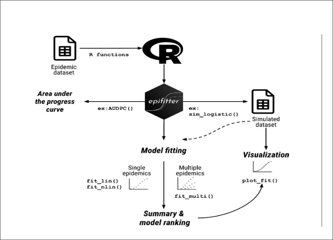
7.2 Epifitter package
The epifitter package (Figure 9) allows working with actual or synthetic (simulated) DPCs for single epidemics or replicated experimental data (Alves and Del Ponte 2021). Epifitter provides a set of tools for aiding in the visualization, description, and comparison of plant disease progress curve (DPC) data. The software package is accessible for download on CRAN (The Comprehensive R Archive Network) and can be installed by executing the command install.packages(“epifitter”). Once the data are loaded, using the epifitter package functions the following can be done.
fitting and ranking for the models based on summary stats.
comparing model parameters.
calculating the area under the disease progress curve.
plotting diagnostic and publication-ready plots via customization of ggplot2 objects.

7.3 Workflow of epifitter package
Once the epidemic dataset is collected, its imported in R studio and further analysis is done using the pre installed epifitter package. The built in functions for Model fitting (fit_lin, fit_nlin, and fit_nlin2) is used to fit the epidemic dataset into different statistical model to identify the best fit model that describes the overall epidemiological process. For making a simulated dataset of the disease severity rating with time, four functions (sim_logistic, sim_exponential, sim_monomolecular, sim_gompertz) specifically designed for the four statistical models are used. The further analysis and visualization can be done using the simulated dataset. For comparative study between different treatments and variables in the disease progression studies, a quantitative summary of the overall epidemiology can be understood using the Area Under Disease Progress Curves (AUDPC()), and its mathematical modification Area under Disease Progress Stairs (AUDPS()) function can be used. These two functions provide a quantitative summary on the disease progress (Alves and Del Ponte 2021). The complete analytical pipeline of the epifitter package- from data input to model fitting, visualization, and summary, is illustrated in Figure 10. This workflow diagram provides a structured overview of the package’s core functions and their sequential application in epidemic data analysis. A key limitation of the epifitter package is that its modelling accuracy depends on sufficiently detailed and regularly spaced epidemic observations, and the assumptions embedded in each growth model may reduce reliability when datasets are sparse, irregular, or highly variable.
| Function | Description |
|---|---|
fit_lin() |
Fits models to single DPC data via linearization |
fit_nlin() |
Fits models to single DPC via nonlinear regression |
fit_nlin2() |
An extension of fit_nlin() that allows estimating the maximum asymptote parameter \(K\) |
fit_multi() |
Fits models to multiple DPCs using either linear or nonlinear regression |
plot_fit() |
Generates ggplot2 visualization of the output from a model-fitting object |
sim_exponential() |
Simulates DPC using the exponential model |
sim_monomolecular() |
Simulates DPC using the monomolecular model |
sim_logistic() |
Simulates DPC using the logistic model |
sim_gompertz() |
Simulates DPC using the Gompertz model |
AUDPC() |
Calculates the area under the disease progress curve |
AUDPS() |
Calculates the area under the disease progress stairs |
8 AUDPC
Disease severity in any plant-patho system can be assessed either once at the peak of the epidemic or several times at some intervals starting from disease initiation until the end of the epidemic. The former method of assessment measures the cumulative effects of all the factors operating during the course of epidemic viz. the terminal disease severity scores (TDS), while the latter can be used to estimate different parameters like the area under the disease progress curves (AUDPC) (Mukherjee, Mohapatra, and Nayak 2010). The area under the disease progress curve (AUDPC) is a useful quantitative summary of disease intensity over time, for comparison across years, locations, or management tactics. The most commonly used method for estimating the AUDPC, the trapezoidal method (Figure 11), is to discretize the time variable (hours, days, weeks, months, or years) and calculate the average disease intensity between each pair of adjacent time points (Madden, Hughes, and Van den Bosch 2007). The AUDPC summarizes the “total measure of disease stress” and is largely used to compare epidemics (Jeger and Viljanen-Rollinson 2001). In the context of disease progression analysis, we can delineate the time points as a sequence (ti), where the temporal intervals between consecutive points may exhibit either uniformity or variability. Concurrently, we are presented with corresponding disease severity metrics (yi). Here, we establish y(0) = y0 as the baseline infection or disease level at t = 0, denoting the initial observation of disease severity in our investigation. A(tk), referred to as the Area Under the Disease Progression Curve (AUDPC) at t = tk, represents the cumulative disease severity up to t = tk, and is formulated as the integral of the disease severity over the time period (Mukherjee, Mohapatra, and Nayak 2010).
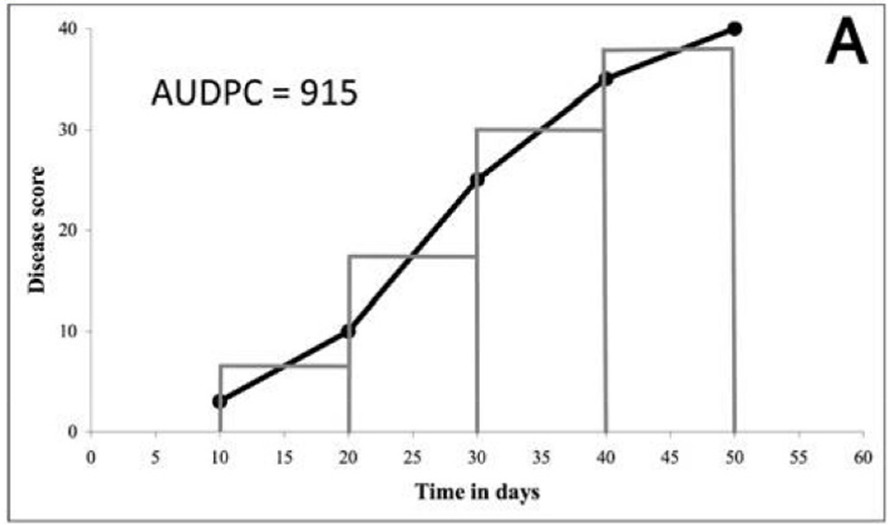
\[\mathrm{AUDPC} = \sum_{i=1}^{n-1} \frac{(y_i + y_{i+1})}{2}\,(t_{i+1} - t_i) \tag{10}\]
yi : Assessment of a disease (percentage, proportion, ordinal score, etc.) at the ith observation
ti : Time (in days, hours, etc.) at the ith observation
n : Total number of observations.
This approach of summarising disease progress data into one value is appropriate when damages to host are proportional to the total amount and duration of the disease. When observed disease patterns can be fitted satisfactorily to a model, then AUDPC can be directly obtained from the model intergated over time (Jeger and Viljanen-Rollinson 2001). When we compare different epidemics, it may be necessary to standardise AUDPC values in order to take into account the fact that epidemics may differ in their lengths of duration. A standardised AUDPC value is obtained by dividing the AUDPC by the total duration time and sometimes by the integration interval (t).
9 AUDPS
The first observation typically indicates the initial level of disease, while the last observation reflects the final extent of the disease at the end of the assessment period. Both of these points are crucial for understanding the full trajectory of disease progression. If these observations are undervalued, the overall assessment may not accurately reflect the severity or impact of the disease over time. The AUDPS method addresses the limitations of AUDPC by giving greater weight to the first and last observations in a disease assessment, which are often undervalued in the AUDPC calculation. This improvement, which results in a better estimation of the overall impact of a disease over time, is particularly important in studies of plant-pathogen interactions, where understanding the full extent of disease progression is essential for effective management (Simko and Piepho 2012).
10 Conclusion
Disease progress curves (DPCs) - derived from repeated measurements of disease incidence or severity over time - are invaluable tools in agricultural epidemiology that encapsulate the dynamic interplay of host, pathogen, and environment throughout an epidemic. By fitting classical growth-curve models such as Exponential, Monomolecular, Logistic, or Gompertz to these temporal data, researchers can obtain biologically meaningful parameters (e.g., initial inoculum level, infection rate) that facilitate rigorous comparisons between epidemics under different conditions or management strategies. The use of summary metrics such as AUDPC and AUDPS further enables succinct quantification of overall disease burden supporting comparisons across seasons, treatments, or cultivars. The integration of open-source statistical software such as epifitter in R - which streamlines model fitting, simulation, visualization, and summary calculation - greatly enhances accessibility, reproducibility, and interpretability of disease‐progress analyses. Nevertheless, to fully realize the potential of DPC-based epidemiology in modern agroecosystems, future work should strive for more comprehensive frameworks that combine classical modeling with emerging assessment technologies (e.g., remote sensing, high-throughput phenotyping) and account for environmental variability, host genetic heterogeneity, and management interventions. Such integrated approaches will improve both predictive power and decision-support capacity ultimately aiding timely, effective disease management and contributing to crop health and food security.
References
Publication Information
- Submitted: 10 December 2025
- Accepted: 17 December 2025
- Published (Online): 19 December 2025
Reviewer Information
Reviewer 1:
AnonymousReviewer 2:
Anonymous
The statements, opinions and data contained in all publications are solely those of the individual author(s) and contributor(s) and not of the publisher and/or the editor(s).
The publisher and/or the editor(s) disclaim responsibility for any injury to people or property resulting from any ideas, methods, instructions or products referred to in the content.
© Copyright (2025): Author(s). The licensee is the journal publisher. This is an Open Access article distributed under the terms of the Creative Commons Attribution-NonCommercial-NoDerivatives 4.0 International License, which permits non-commercial use, sharing, and reproduction in any medium, provided the original work is properly cited and no modifications or adaptations are made.