
Advancing Crop Improvement through Honeycomb Selection Design: Principles, Statistical Frameworks, Software Tools, and Applications: A Review
Field evaluation of genotypes is confounded by soil heterogeneity and interplant competition, which inflate error and lower the heritability of yield traits. The Honeycomb Selection Design (HSD), conceived by A. C. Fasoulas and refined by Tokatlidis and co-workers, evaluates individual plants in a Read more …

Field evaluation of genotypes is confounded by soil heterogeneity and interplant competition, which inflate error and lower the heritability of yield traits. The Honeycomb Selection Design (HSD), conceived by A. C. Fasoulas and refined by Tokatlidis and co-workers, evaluates individual plants in a hexagonal grid at ultra-wide spacing, comparing each plant with a moving ring of equidistant neighbours under nil competition. This review synthesises HSD’s principles, geometry and statistical framework, and compares it with conventional designs and spatial mixed models. It examines selection indices, the rhoneycomb R package and recent doubts about the homeostasis index. Applications in sunflower, barley, durum wheat, lentil and alfalfa are summarised, along-side long-term evidence from rice, mungbean and cotton. Limitations include land requirement, dependence among overlapping ring-adjusted values, and extrapolation to dense stands. Integration with UAV phenotyping, spatial mixed models, genomic prediction and microbiome-assisted selection offers the most promising route to climate-resilient cultivars.
Spatial heterogeneity, Homeostasis index, Intra-cultivar variation, Stress tolerance, Root-zone microbiome, Plant yield efficiency
1 Introduction
Global crop output must rise substantially while limiting environmental costs, yet current yield trends fall short of the doubling needed by 2050 (Ray et al. 2013; Tilman et al. 2011). Climate trends since 1980 have already depressed maize and wheat yields in many regions (Lobell et al. 2011), so genetic gain for abiotic stress tolerance must become faster and more precise (Mickelbart et al. 2015; Hickey et al. 2019), with rapid breeding and varietal replacement especially critical in developing regions (Atlin et al. 2017). The reliability of selection, which rests on the quality of field experimentation, therefore underpins the whole breeding pipeline.
The response to selection depends on selection intensity, genetic variance and heritability, so any non-genetic variation in the selection unit slows genetic gain. Sound experimental design improves precision by minimising error and accounting for external sources of variation (Casler 2015), through replication, blocking, lattice and alpha designs (Patterson and Williams 1976) and, more recently, spatial mixed models (Gilmour et al. 1997; Rodríguez-Álvarez et al. 2018). Plot-based designs nevertheless remain constrained by soil and microenvironmental heterogeneity and by competition within dense plots, particularly in perennial and outcrossing species. Both reduce the heritability of yield traits (Fasoula and Tokatlidis 2012). Heritability governs the expected response to selection (Falconer and Mackay 1996), and its estimation from field data depends on how error and replication are modelled (Holland et al. 2003; Piepho and Möhring 2007). Competition adds a further source of bias: neighbouring genotypes that differ in vigour or height alter each other’s environment, which distorts yield comparisons in small, unbordered plots (Rebetzke et al. 2014). Because competition among plants is typically size-asymmetric, larger individuals obtain a disproportionate share of resources (Weiner 1990). Competition can even outweigh soil heterogeneity (Fasoulas and Fasoula 1995) and may favour competitive rather than productive genotypes (Donald 1968; Tokatlidis 2022).
The Honeycomb Selection Design (HSD) was proposed by A. C. Fasoulas and advanced by Tokatlidis and collaborators (Fasoulas and Fasoula 1995; Fasoula and Tokatlidis 2012). It evaluates individual plants grown under greatly reduced competition, placed in triangular or hexagonal configurations so that every plant has equidistant neighbours and can be compared directly with them (Fasoula and Fasoula 2000). It is especially valuable in early segregating generations, where variability is high, seed is limited and replicated plots are difficult to manage (Fasoula and Tokatlidis 2012). Its use has since expanded to stress tolerance assessment, yield stability, selection within released cultivars and plant–microbiome studies under field conditions.
2 Principles and defining features of the Honeycomb Selection Design (HSD)
HSD combines experimental design with plant selection. Genotypes are placed at predetermined positions in a hexagonal pattern in which each plant has six equally spaced neighbours, and control entries are distributed regularly according to the design parameter K. Field variability is thereby measured directly rather than managed only by randomisation (Fasoulas and Fasoula 1995). Its defining features are:
· Individual plants, not plots, are the units of experimentation and selection.
· Genotypes follow a systematic triangular or hexagonal pattern instead of random allocation.
· Control entries are spread uniformly, at fixed positions determined by K, so that field variability can be measured effectively.
· Ultra-wide spacing minimises competition for light, water and nutrients, so each plant can express its genetic potential.
· Selection of individual plants within superior genotypes is supported, which is useful in early generations and under stress.
Together, wide spacing and systematic replication allow genetic differences to be assessed more accurately than in dense planting designs, where competition and soil heterogeneity obscure genotype performance (Katsileros et al. 2023).
3 Theoretical foundations: competition, nil-competition and the productive ideotype
3.1 Classification of interplant competition
HSD rests on a four-type classification of interplant competition according to how neighbours share resources (Fasoula 1990; Fasoula and Fasoula 2000). Allo-competition is unequal sharing arising from both genetic and environmental differences; auto-competition is unequal sharing arising only from environmental or acquired differences; iso-competition is equal sharing, which is rarely achieved; and Nil-competition is best understood as a practical growing condition in which competition among plants is reduced to a level that has little influence on their performance, a state that HSD approximates through wide and uniform plant spacing.
3.2 Six conditions for maximising genetic gain
Fasoula and Fasoula (2000) distilled six interrelated conditions for maximising genetic gain through phenotypic selection: (1) evaluation without competition; (2) fixation of favourable genes, achieved naturally in self-pollinated species and through controlled selfing and wide spacing in cross-pollinated, biennial, perennial or clonal crops; (3) multi-environment screening across years to capture genotype by environment interactions and diverse stresses; (4) systematic honeycomb geometry; (5) yield-component analysis of single plants under nil-competition; and (6) continued selection within cultivars after release, to exploit beneficial mutations and epigenetic changes, eliminate harmful ones and prevent yield decline during seed multiplication.
3.3 Nil-competition and the productive ideotype
The rationale for nil-competition extends beyond statistical convenience. (Donald 1968) distinguished the competitive plant from the communal ideotype suited to a crop community. Selection under intergenotypic competition can make the competitive ideotype falsely selectable, whereas the productive ideotype, which combines low competitiveness with high plant yield efficiency (PYE), becomes selectable only when widely spaced individuals prevent plant-to-plant interference (Tokatlidis 2022). In maize, hybrids that depend on high plant populations are unstable when density or stress varies (Tokatlidis and Koutroubas 2004), and breeding gains in maize have come largely through improved stress tolerance, including tolerance of high plant density (Duvick 2005). HSD provides the field arrangement in which PYE can be measured and selected without interference from neighbours.
4 Classification, geometry and construction of honeycomb selection designs
4.1 Single entry design (HSD0)
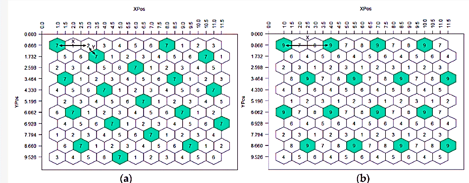
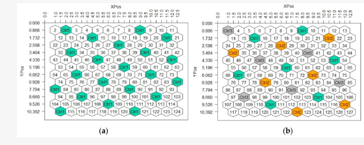
In HSD0, a single genotype is represented by a large number of plants, all of which are selectable. Optionally, one or three control entries are distributed through the grid to sample heterogeneity, so that every plant can be compared with a nearby, standardised reference (Figure 1).
4.2 Multiple entry design, HSD(E)
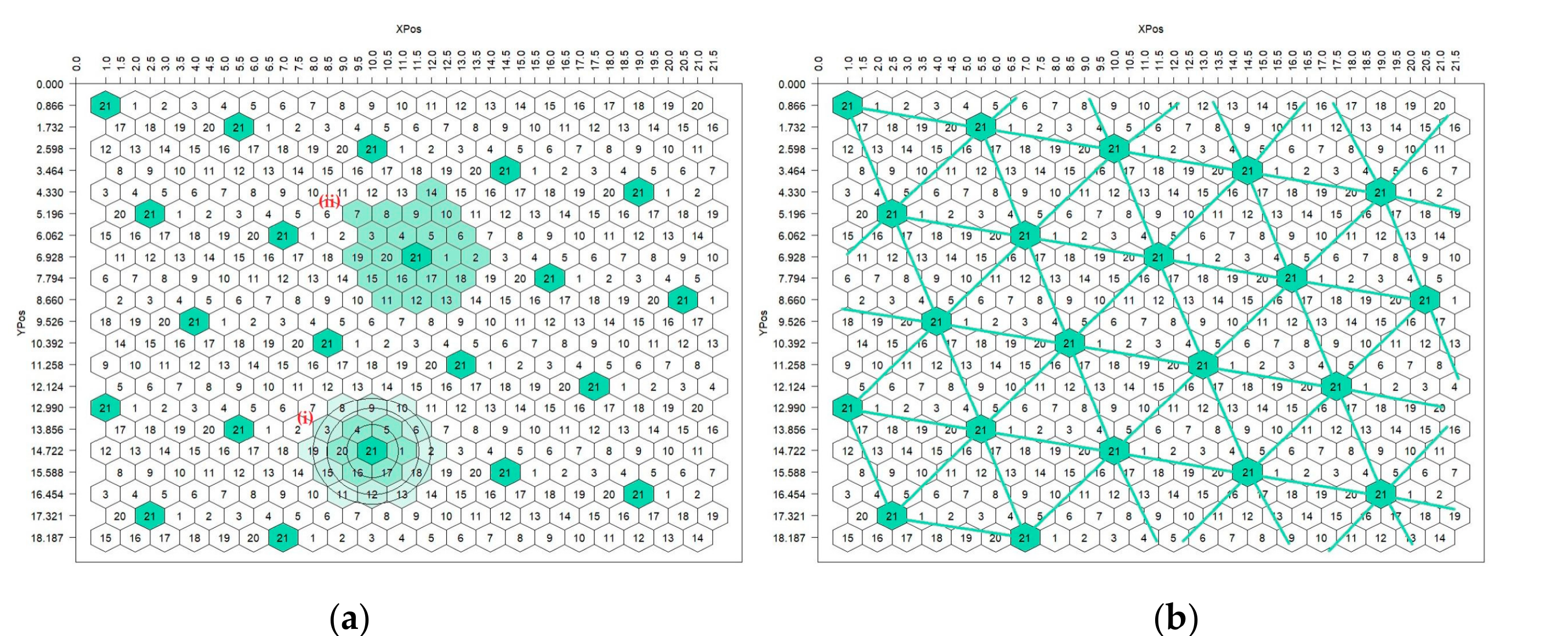
The multiple-entry design, HSD(E), evaluates several genotypes simultaneously. Entries follow coordinate steps X (horizontal) and Y (diagonal) (Figure 2), and the layout is grouped or ungrouped depending on whether X and Y share common divisors. Each plant is again surrounded by six neighbours. The number of entries, E, is fixed by the coordinates:
\[ E = X^2 + XY + Y^2 \]
where X and Y are non-negative integers that are not both zero. Designs with 7 and 21 entries are denoted HSD(7) and HSD(21), respectively (Table 1). This is the same notation as the R-7, R-21, R-57 and R-133 designs of Fasoula and Fasoula (2000): R-7 and HSD(7) denote the same layout. The number of replications per entry is set by the breeder according to the genetic variation among entries and the variability of the field, with more replication where material is diverse or the field is uneven (Katsileros et al. 2023).
| X | Y | E = X2 + XY + Y2 | Designation |
|---|---|---|---|
| 1 | 1 | 3 | HSD(3) |
| 2 | 1 | 7 | HSD(7) |
| 3 | 1 | 13 | HSD(13) |
| 4 | 1 | 21 | HSD(21) |
| 5 | 1 | 31 | HSD(31) |
| 7 | 1 | 57 | HSD(57) |
| 11 | 1 | 133 | HSD(133) |
4.3 Layout construction using coordinate geometry
Layouts are built by coordinate geometry. K is an integer design parameter that, for a given number of entries E, K does not change the number of entries E or the systematic hexagonal pattern; it changes where each entry starts in each row. It fixes the initial entry number of each field row and hence where each entry falls (for example, K = 2 in the rhoneycomb call HSD(7, 2, 12, 12, 1)); in single-entry designs with controls, K (1, 3, 5 or 7) fixes which plots carry the controls. Different K values shift entry positions but do not change the even, systematic arrangement, so any K available for a design may be used. How far apart plants of the same entry lie is set by X and Y (Figure 1), and every entry occupies the centre of a moving ring on a triangular grid, which samples spatial heterogeneity in a controlled and repeatable way. Two replication concepts follow (Fasoulas and Fasoula 1995; Katsileros et al. 2023). Type 1, the moving ring(Figure 3), consists of the 6 to more than 120 plants immediately surrounding a given plant, depending on layout and planting density. Type 2, the circular skeleton, is a ring of the size needed to contain the entire set of entries, so that it forms a complete replicate block. Because the ring changes for each plant evaluated, every plant is compared with a local reference rather than the trial mean, which helps separate genetic performance from local growing conditions.
4.4 Field establishment
When d is the spacing between plants within a row, the spacing between rows is 0.866 × d. Plants therefore stand at the corners of equilateral triangles, and an area of 0.866 × d2 is allotted to each. Because each experimental unit is a single plant, one seed per position is generally sufficient, although two or three may be sown and thinned later. The absence of competition and border effects means that missing plants cause little concern, keeping establishment and analysis straightforward.
5 Controlling Field Heterogeneity: The Honeycomb Method in Comparative Perspective
5.1 Historical approaches to local control
Plant breeding seeks both the best individual plants within an entry (for example F₃ lines from a single cross) and the best entries within a group. According to (Fasoulas and Fasoula 1995), within-entry selection was long considered unreliable because field variability concealed genetic differences, although competition in dense populations can affect selection efficiency even more than soil heterogeneity. HSD was developed by combining and improving the most effective features of four earlier approaches, which are summarised here as described by Fasoulas and Fasoula (1995; see also (Fasoula and Fasoula 2000)):
Contiguous control method: A standard cultivar was placed beside each plot and plot performance expressed relative to it. It reduced the influence of soil variation but needed many control plots, because correlation between neighbouring plots declines rapidly with distance.
Moving-average method: Each plot was compared with the mean of its surrounding plots, controlling variability without additional land provided plots were randomly arranged.
Method of correlated traits: Selection used more heritable secondary traits, such as ear prolificacy in maize, but their relationship with yield changed across environments and genetic backgrounds.
Grid method: The field was divided into smaller sections and the best plants or genotypes selected within each, which gave gradual, consistent yield gains in maize mass selection.
Formal neighbour-based models grew out of these ideas (Bartlett 1978; Wilkinson et al. 1983; Besag and Kempton 1986) and were later recast as linear variance models within the mixed-model framework (Piepho et al. 2008).
5.2 The honeycomb method
The honeycomb method drew on all four approaches while avoiding their weaknesses. Like the moving-average method it uses a local reference, but each plant is evaluated against a hexagonal group of equally spaced neighbours, and its yield is expressed relative to the mean of this ring. The ring size can be adjusted to soil variability, genetic diversity and population size. Because the ring is calculated separately for each plant and all entries are surrounded by the same type of neighbours, within-entry selection is expected to remain effective irrespective of trial size or number of locations.
5.3 HSD relative to conventional and modern spatial approaches
Modern field trial analysis has developed along three lines. Incomplete block designs, such as lattices and resolvable alpha designs, recover information by blocking plots (Patterson and Williams 1976). Augmented and partially replicated layouts adjust unreplicated test lines against replicated checks (Federer and Raghavarao 1975), and early-generation trials with correlated data have been formulated within mixed models (Cullis et al. 2006). Resolvable row–column designs can be improved further by adding one- or two-dimensional spatial components such as linear variance models (Piepho and Williams 2010), and two-dimensional spatial error structures were introduced for field experiments by (Cullis and Gleeson 1991). (Lado et al. 2013) used a moving mean of neighbouring plots as a covariate, which is conceptually close to the honeycomb ring. Spatial analysis has progressed from nearest neighbour analysis (Wilkinson et al. 1983) to separable autoregressive error structures (Gilmour et al. 1997) and smooth surfaces fitted with penalised splines (Eilers and Marx 1996; Velazco et al. 2017; Rodríguez-Álvarez et al. 2018). Spatial adjustment increased genomic prediction accuracy in wheat (Lado et al. 2013), and linear mixed models are now standard for crop variety evaluation (Smith et al. 2001).
HSD therefore differs not by ignoring spatial variation but by addressing it within the layout itself, giving each plant its own local reference while removing competition at source. Mixed-model methods correct heterogeneity at the analysis stage and typically operate on plot means grown at competitive densities (Table 2).
| Approach | Basis for controlling heterogeneity | Selection unit | Main strengths | Main limitations |
|---|---|---|---|---|
| Blocked and incomplete-block designs (RCBD, lattice, alpha) | Blocking and randomised replication | Plot | Unbiased error estimation; widely implemented | Seed needed for replication; plot-level competition persists |
| Augmented and partially replicated designs | Replicated checks used to adjust unreplicated entries | Plot or row | Accommodates many entries with limited seed | Adjustment depends on how well checks sample field variation |
| Neighbour-based and spatial mixed models (nearest-neighbour, AR1×AR1, P-splines) | Covariates, correlated errors or smooth surfaces fitted at analysis | Plot | Flexible modelling of trends; improved selection accuracy | Requires model selection and software; competition among plants not removed |
| Honeycomb Selection Design | Systematic hexagonal grid; moving-ring local reference; regular controls; nil-competition | Individual plant | Competition removed; each plant has its own reference; many plants per entry; missing plants tolerated | Large land and labour per entry; extrapolation to dense stands and index assumptions need validation |
5.4 Statistical advantages of HSD
Because each entry is represented by many plants, entry means can be compared by t-tests based on each entry’s own error estimate rather than a pooled error term, and unequal numbers of plants cause no major analytical difficulty, subject to the dependence caveat discussed below. The ability of the honeycomb design to capture spatial variation has been compared with conventional designs using maize and wheat breeding trial data (Tokatlidis 2016).
Entry-specific t-tests treat plants as independent observations. In an HSD, however, soil variation is spatially correlated and the moving rings of adjacent plants overlap, so the ring-adjusted values of neighbouring plants may be dependent. Positive dependence of this kind can lead to underestimated standard errors if it is ignored (Cullis and Gleeson 1991; Gilmour et al. 1997). Welch’s (Welch 1947) and Cochran’s (Cochran 1964) approximations accommodate unequal variances but not dependence among plants, so a spatial error model, or a simulation under no true entry differences, would be a useful check on the nominal error rate. This limitation is also listed in Table 5.
6 Statistical framework for selection
6.1 Selection indices
Selection in an HSD experiment uses indices of yield performance and stability: PYE, the homeostasis index (HI), the plant and entry predictive equations (PPE and EPE), the entry yield index (EYI) and the coefficient of response to selection (CRS) (Katsileros et al. 2023). Their formulae and purposes are summarised in Table 3. HI is calculated at the entry level, from the mean and standard deviation of all plants of an entry within a trial (E_HI in rhoneycomb output), and mPYE and mPPE are the entry means of the plant-level PYE and PPE values.\(PYE = \left(\frac{x}{\overline{x}_r}\right)^2\)
| Index | Formula | Purpose |
|---|---|---|
| Plant Yield Efficiency (PYE) | \(PYE = \left(\frac{x}{\overline{x}_r}\right)^2\) | Measures a genotype’s yield response at nil-competition; \(x\) is the yield of the central plant and \(\overline{x}_r\) the mean yield of its moving ring. |
| Homeostasis Index (HI) | \(HI = \left(\frac{\overline{x}}{s}\right)^2\) | Assesses a genotype’s yield stability under environmental variation, from its entry mean (\(\overline{x}\)) and standard deviation (\(s\)), both computed over all plants of the entry within a trial (entry level; E_HI in rhoneycomb). |
| Plant Predictive Equation (PPE) | \(PPE = PYE \times HI\) | Combines an individual plant’s yield response and stability into a single predictive score. |
| Entry Predictive Equation (EPE) | \(EPE = EYI \times HI\) | Entry-level counterpart of PPE; the Entry Yield Index (EYI) is the squared ratio of the entry mean to the grand trial mean, \(EYI = \left(\frac{\overline{x}}{\overline{x}_t}\right)^2\). |
| Coefficient of Response to Selection (CRS) | \(CRS = \frac{\overline{x}_{sel} - \overline{x}_{contr}}{s}\) | Evaluates germplasm potential by comparing the mean yield of the top-selected plants with that of an entry control, scaled by the standard deviation. |
| Mean Plant Yield Efficiency (mPYE) | \(mPYE = \frac{1}{n}\sum_{i=1}^{n} PYE_i\) | Entry-level yield response; used to rank entries by yield when the aim is to identify high-yielding entries. |
| Mean Plant Predictive Equation (mPPE) | \(mPPE = \frac{1}{n}\sum_{i=1}^{n} PPE_i\) | Entry-level counterpart of PPE; ranks entries on yield response and stability combined. |
6.2 Two-stage selection procedure
Selection proceeds in two stages. First, entries are ranked by yield (mean yield, EYI or mPYE), stability (HI) or both (EPE or mPPE), depending on whether the entries are highly heterogeneous or fairly homogeneous; when the aim is to evaluate germplasm as starting material, entries are ranked by CRS against a selected control genotype. Second, within the top entries, individual plants with high PYE are selected (Katsileros et al. 2023). In principle, quantitative genetic theory predicts that the expected response depends on the selection differential and heritability (Falconer and Mackay 1996), and heritability should rise when competition and spatial noise are removed from the phenotypic variance; direct comparisons of heritability under HSD and conventional designs have yet to be reported.
6.3 Critical evaluation of the homeostasis index
The usefulness of these indices rests on an assumption that is rarely examined: that the coefficient of variation (CV) of individual plant yields reflects a genotype’s ability to perform consistently among plants, so that HI, based on the inverse of CV, measures stability. (Tokatlidis et al. 2023) tested whether CV declines with increasing mean yield, as expected from Taylor’s power law (Taylor 1961), in several single-plant honeycomb trials. In most, particularly those with strong spatial variation and high overall CV, variance was closely related to mean yield, which could change HI values even when stability had not changed; adjusting variance for its dependence on the mean did not confirm the expected negative relationship. The authors advised interpreting HI with care, because unvalidated use could wrongly raise or lower the ranking of a progeny line, and suggested checking the variance in each trial and, where needed, calculating HI from a transformed variance. The honeycomb framework is thus still being evaluated and improved.
HI also differs from the stability concepts of classical multi-environment analysis, which describe how performance changes along an environmental gradient (Finlay and Wilkinson 1963; Eberhart and Russell 1966). HI is computed from among plant variation within a trial. The two notions are related but not interchangeable, which reinforces the need for multi-environment screening (Section 3.2).
6.4 Relationship to mixed-model evaluation
Because HSD generates many observations per entry, entry means can be estimated precisely and, in principle, analysed in linear mixed models with spatial terms (Smith et al. 2001; Gilmour et al. 1997). Comparing honeycomb index rankings with mixed-model predictions across crops and environments would show where the approaches agree and where each adds information. Such models can be fitted in R, for example with generalised least squares and an exponential spatial correlation structure in the nlme package (Pinheiro and Bates 2000) or with penalised spline surfaces in SpATS (Rodríguez-Álvarez et al. 2018), using the plant coordinates that the honeycomb layout already provides.
8 Applications of honeycomb selection design
HSD is used to select superior plants in early generations such as F2, to develop varieties for drought, salinity and low-input conditions, to improve existing cultivars by intra-cultivar selection and to enhance yield and stability. It has also been applied to root trait and plant–microbiome studies, because wide spacing allows natural root development (Fasoula et al. 2020). Five case studies (Table 4) span cereals, an oilseed, a pulse and a forage crop.
| Crop and trait | Design features | Key outcome |
|---|---|---|
| Sunflower, disk area and yield | Five genotypes; honeycomb selection for largest disk area at 1.3 m between furrows and 1.5 m between plants (about 0.51 plants m-2); original and selected genotypes compared under three plant densities (5.3, 6.7 and 8.9 plants m-2). | Across the five genotypes, selected populations had larger disk areas (about 415 vs 312 cm2) and higher seed yield (about 7.65 vs 5.49 t ha-1) than the originals at each density (means calculated from Tables 3 and 5 of (Ibrahim and Abdulhamed 2024)); only the direction of the yield effect is given, because the source reports implausibly high yields and internal inconsistencies). |
| Barley, BYDV-PAV resistance and stress buffering | Replicated honeycomb layout at 1.2 plants m-2; five cultivars and two Tunisian landraces; divergent single-plant selection over two cycles. | High-yielding lines showed strong virus resistance and suppressed yield loss under inoculation; selected lines retained biomass buffering capacity under dense, multi-environment stands (Ben Ghanem et al. 2018; Tsivelikas et al. 2022). |
| Durum wheat, grain yield and protein content | Honeycomb trials under ultra-low density within two commercial cultivars; divergent selection for yield and protein content simultaneously. | Exploitable within-cultivar variation identified; progeny lines combined above-average yield and protein content at commercial density (Ninou et al. 2022). |
| Lentil, molecular verification of sister lines | Honeycomb design at 1.2 plants m-2 (about 1 m between plants); three successive generations of honeycomb pedigree selection within the Greek landrace Evros; 40 sister lines, 15 SSR markers. | Low differentiation between consecutive generations (2.5% and 7.7%) but 26.7% between first and third; 88% of variation within generations; 14 of 48 alleles (29.2%) lost over two cycles, and allelic composition shifted (Gleridou et al. 2022). |
| Alfalfa, root-zone bacterial diversity | Honeycomb layout (called the R0 design in the source), 20 rows × 35 plants per row, 1 m interplant spacing; four Medicago genotypes (three with wild-relative backgrounds, one commercial cultivar), field-grown for six months. | Root-zone bacterial assemblages differed significantly by genotype and from bulk soil; specific taxa were positively associated with forage yield (Omirou et al. 2024). |
8.1 Foundational and comparative evidence
Fasoula and Fasoula (2000) proposed honeycomb breeding as a universal approach applicable to all four major cultivar types: inbred lines, hybrids, clones and populations. Using rice, maize, potato and alfalfa, they showed that the same principles apply: plants are grown at wide, uniform spacing from the earliest generation and selected for yield per plant, stress tolerance and response to inputs; promising material then enters larger replicated honeycomb trials such as R-7, R-21, R-57 and R-133; and selection continues after cultivar release.
In rice, plants selected at very low density from a single F2 population of the commercial rice hybrid ‘1992’ (introduced to Greece from the United States) and advanced to F6 gave the cultivar Olympiad (Danos, 1998, cited in (Fasoula and Fasoula 2000)). In randomized complete block trials over two years (1994–1995) it out yielded its parent hybrid (by 8%) and the best local check in grain yield and most quality traits, showing that selection for high, consistent performance without competition can also improve tolerance of stresses met at normal densities. It was released in the F6 generation, after six generations counting from the F₁ hybrid, compared with the 12 to 14 generations needed with conventional methodology (Fasoula and Fasoula 2000), which points to faster cultivar development in self-pollinated crops; speed breeding offers a complementary route (Watson et al. 2018). In mungbean, honeycomb-derived lines yielded more and gave more superior lines than pedigree, single-seed descent or bulk selection (Gill et al. 1995). In cotton, honeycomb selected lines outperformed pedigree and single-seed descent lines for seed cotton yield, boll weight and fibre length (Batzios, 1997, cited in (Fasoula and Fasoula 2000)), and the best lines came from only a few outstanding F2 plants. Honeycomb selection can therefore identify superior individuals at very early generations, when single-plant selection is usually considered unreliable.
8.2 Abiotic stress tolerance and trait improvement
Selecting for abiotic stress tolerance in segregating populations is difficult because stress expression is spatially heterogeneous and phenotyping helps breeders only when it is relevant to the target environment (Passioura 2012; Richards 2006). In sunflower, Ibrahim and Abdulhamed (2024) selected five genotypes (Aqmar, Haisin, Ishaqi, Sakha and Flami) over successive cycles for the largest disk area, with 1.3 m between furrows and 1.5 m between plants (about 0.51 plants m-2), and compared selected and original populations at three densities (5.3, 6.7 and 8.9 plants m-2). Averaged over the five genotypes, the selected populations had larger disk areas (about 415 against 312 cm2) and higher seed yield (about 7.65 against 5.49 t ha-1) than the originals, and out-yielded them in every genotype and density combination (Ibrahim and Abdulhamed 2024). Absolute seed yields are not quoted, because the values reported in the source are implausibly high for sunflower and other tables in that paper contain internal inconsistencies; only the direction of the effect is used here. The study shows how HSD can be combined with density trials, but the result is indicative: the means are calculated here from Tables 3 and 5 of the source, other tables in that paper contain internal inconsistencies, and its density comparison was a split-plot randomized complete block trial rather than a honeycomb layout.
8.3 Intra-cultivar selection in barley and durum wheat
Intra-cultivar selection exploits the genetic variation that remains within commercial cultivars. In barley, (Ben Ghanem et al. 2018) selected plants within cultivars and found lines with much higher resistance to Barley yellow dwarf virus-PAV (BYDV-PAV); two lines of the cultivar Imen lost no more than 10% of yield after infection, similar to the resistant check, whereas yield loss reached around 60% under severe inoculation. (Tsivelikas et al. 2022) tested first- and second-cycle lines at normal farming densities in three semi-arid Mediterranean environments. Genotypes differed significantly for several agronomic and physiological traits and biological yield was stable across environments; lines selected for high yield at ultra-low density also performed well in dense stands, whereas lines selected for low yield generally performed poorly, indicating a strong link between performance at ultra-low and normal densities. In durum wheat, (Ninou et al. 2022) selected plants of the cultivars Svevo and Maestrale for both grain yield and protein content at ultra-low density; at normal density several selected lines were superior for both traits, a faster and more economical alternative to developing new varieties. Single-plant selection at ultra-low density has also been used to test for intra-cultivar variation in seed protein and oil content in soybean (Fasoula and Boerma 2005).
8.4 Molecular verification in lentil and root-zone bacterial diversity in alfalfa
Although honeycomb breeding relies on phenotypic rather than marker-based selection, it also produces measurable genetic change. (Gleridou et al. 2022) analysed sister lines from successive cycles of honeycomb pedigree selection in the lentil landrace Evros with simple sequence repeat (SSR) markers. Differentiation between consecutive generations was low (2.5% between the first and second, 7.7% between the second and third) and 88% of the variation lay within generations, but the first and third generations differed more (26.7%). Fourteen of the 48 alleles found in the first generation (29.2%) were lost over two cycles, although some of this apparent loss may reflect heterozygous HRM profiles segregating out (heterozygosity in lentil is very low), and allelic composition shifted, so markers can be used to monitor selection response and manage diversity.
The rhizosphere microbiome is increasingly recognised as a determinant of plant health (Berendsen et al. 2012). Rhizosphere communities can be heritable in maize under field conditions (Peiffer et al. 2013). In Arabidopsis thaliana, soil type was the main determinant of root-associated bacterial communities, with a smaller but detectable contribution from host genotype (Lundberg et al. 2012; Bulgarelli et al. 2012). Studying such interactions in single plants requires that neighbours do not blur the root zone, a natural strength of widely spaced honeycomb layouts. Omirou et al. (2024) grew four Medicago genotypes in an HSD trial at 1 m spacing: two M. sativa × M. arborea hybrids, one M. sativa nothosubsp. varia breeders’ line (genotype 13) and one commercial M. sativa cultivar. Genotype significantly influenced forage yield and bacterial community composition: genotype 13 had a distinct bacterial assemblage and the lowest forage productivity (Omirou et al. 2024), whereas the abundances of Sphingomonas, Flavisolibacter and Stenotrophomonas were positively correlated with forage yield across the genotypes. HSD is thus an effective platform for plant–microbiome studies, and root-zone microbiome traits could complement alfalfa (Medicago sativa) breeding.
9 Strengths, limitations and research gaps
The evidence reviewed above supports HSD as a rigorous framework for single-plant evaluation, but its assumptions and practical demands constrain its use. Its main strengths are the removal of competition at source, a local reference for every plant, many observations per entry that allow entry-specific error estimates, tolerance of missing plants and an open source implementation. The main limitations, and ways of addressing them, are summarised in Table 5. Much of the evidence reviewed also comes from the originating group and its collaborators, so independent evaluations, where they exist, deserve particular weight.
| Issue | Concern | Suggested way forward |
|---|---|---|
| Land and labour | Ultra-wide spacing and many plants per entry increase the area and handling effort required per entry. | Confine HSD to early-generation and within-cultivar selection, then advance selected material to replicated trials at commercial density. |
| Extrapolation to dense stands | Genotype by density interaction may weaken the link between nil-competition performance and crop level yield (Tokatlidis and Koutroubas 2004). | Include density trials of selected lines, as in sunflower and barley (Tsivelikas et al. 2022) and indicatively, sunflower (Ibrahim and Abdulhamed 2024) |
| Validity of HI | Scale dependence of variance on the mean can distort CV-based stability rankings (Tokatlidis et al. 2023). | Test the variance–mean relationship in each trial and use transformed variance where required; confirm stability in multiple environments. |
| Statistical dependence (pseudo-replication) | Spatially correlated soil variation and overlapping moving rings make ring-adjusted values of neighbouring plants dependent, so entry-specific t-tests may understate standard errors | Check the nominal error rate with a spatial error model or a simulation under no true entry differences (Cullis and Gleeson 1991; Gilmour et al. 1997). |
| Local reference assumptions | Ring-based comparison assumes that heterogeneity is smooth at the scale of the ring; global trends and management effects may remain. | Combine ring references with spatial mixed models (Rodríguez-Álvarez et al. 2018). |
| Breadth of evidence | Reported applications concentrate on a limited set of crops, traits and environments, and most of the evidence comes from the originating group and its collaborators. | Expand independent, multi-location validation across agro-ecologies and crop types, including tropical and subtropical systems. |
Two points deserve emphasis. First, transferability of performance from nil-competition to dense stands is the crux of the method. Results in barley and durum wheat are encouraging, since lines selected at ultra-low density also performed well at commercial densities (Tsivelikas et al. 2022; Ninou et al. 2022), and mungbean and cotton point the same way (Gill et al. 1995; Fasoula and Fasoula 2000). Nevertheless, the relationship between plant density and yield differs among crops and genotypes (Tokatlidis and Koutroubas 2004), so validation at the target density remains good practice. Second, the ring size, which can range from 6 to more than 120 neighbours, is guided by soil variability, genetic diversity and population size; formal criteria for choosing an optimum ring size in different crops would strengthen the method.
10 Conclusions
HSD combines geometric field layout, statistical analysis and plant breeding principles to overcome the two main challenges of single-plant evaluation, soil heterogeneity and interplant competition. Compared with contiguous control, moving average, correlated trait and grid methods, and with plot-based designs analysed at competitive densities, it provides a more direct framework for assessing individual plants. Its quantitative indices, including PYE, HI and CRS, have supported its adoption across cereals, oilseeds, pulses and forage legumes, and they continue to be critically evaluated and refined.
Case studies in sunflower, barley, durum wheat, lentil and alfalfa, together with long-term comparisons in rice, cotton and mungbean, show that the utility of HSD extends beyond conventional yield selection, including its use as a platform for studying plant–microbiome interactions under field conditions. The research agenda most likely to extend its reach in climate-resilient crop improvement comprises validation of nil-competition selection at target densities, combination of honeycomb references with spatial mixed models, and integration with UAV phenotyping and genomic prediction.
Artificial intelligence (AI) tools were used solely for grammatical correction and language improvement. The authors reviewed and verified all content and take full responsibility for the accuracy and integrity of the manuscript.
References
Publication Information
- Submitted: 12 October 2026
- Accepted: 09 November 2026
- Published (Online): 20 November 2026
Reviewer Information
Reviewer 1:
Dr. Gowthaman T
Project Research Scientist- C
ICMR-National Institute of NCD EpidemiologyReviewer 2:
Anonymous
The statements, opinions and data contained in all publications are solely those of the individual author(s) and contributor(s) and not of the publisher and/or the editor(s).
The publisher and/or the editor(s) disclaim responsibility for any injury to people or property resulting from any ideas, methods, instructions or products referred to in the content.
© Copyright (2026): Author(s). The licensee is the journal publisher. This is an Open Access article distributed under the terms of the Creative Commons Attribution-NonCommercial-NoDerivatives 4.0 International License, which permits non-commercial use, sharing, and reproduction in any medium, provided the original work is properly cited and no modifications or adaptations are made.